152 lines
12 KiB
Markdown
152 lines
12 KiB
Markdown
[CGDI] Color Transfer via Discrete Optimal Transport using the *sliced* approach
|
||
==
|
||
|
||
> [name="David Coeurjolly"]
|
||
|
||
ENS [CGDI](https://perso.liris.cnrs.fr/vincent.nivoliers/cgdi/) Version
|
||
|
||
[TOC]
|
||
|
||
---
|
||
|
||
|
||
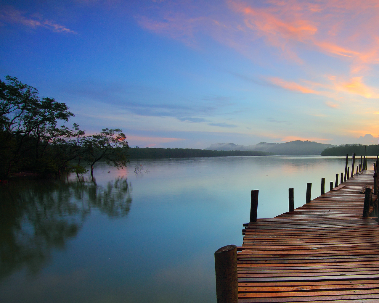
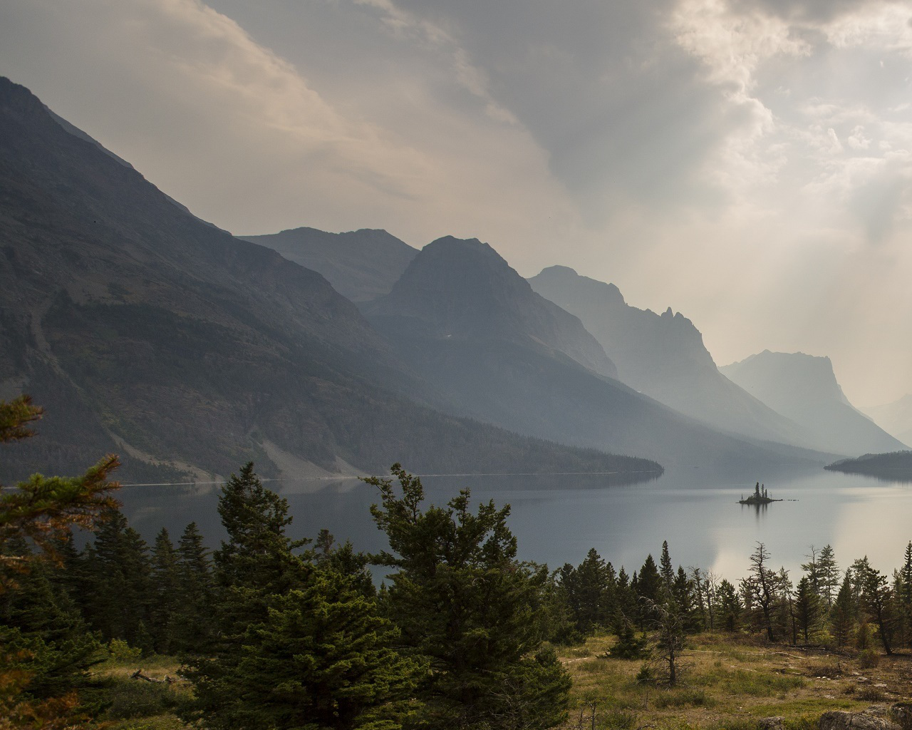
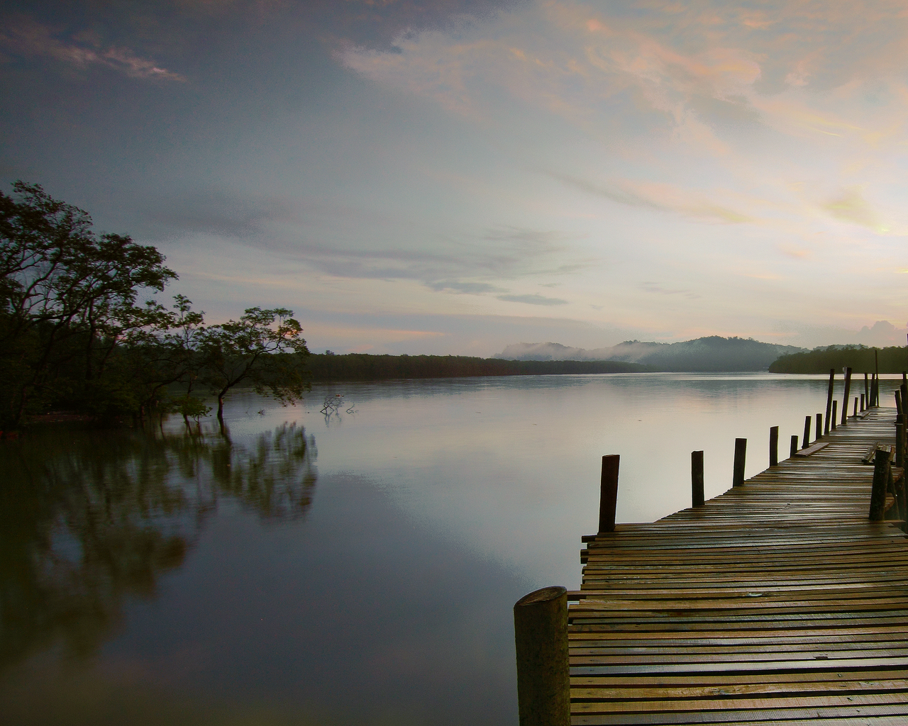
Color transfer is an image processing application where you want to retarget the color histogram of an input image according to the color histogram of a target one.
|
||
|
||
**Example:**
|
||
|
||
Input image | Target image | Color transfer output
|
||
-------|---------|----
|
||
 |  | 
|
||
|
||
|
||
|
||
The idea of this project is to detail a color transfer solution that considers
|
||
the [Optimal Transport](https://en.wikipedia.org/wiki/Transportation_theory_(mathematics)) as a way to *deform* histograms in the most *efficient way* (see below for details).
|
||
|
||
The objective of this TP is to implement a *sliced* approach to solve the color transfer problem via Optimal Transport.
|
||
|
||
# Warm-up 1: Downloading the code
|
||
|
||
The skeleton of the code is available on [this Github Project](https://github.com/dcoeurjo/transport-optimal-gdrigrv-11-2020). This code contains all you need to load and save color images (and to parse command line parameters for the `c++`code). You can download the archive from the Github interface (*"download zip"* menu), or *clone* the git repository. The project contains some `c++` and `python` codes.
|
||
|
||
:::warning
|
||
For python, we encourage you to use the notebooks shared by Vincent on the [CGDI homepage](https://perso.liris.cnrs.fr/vincent.nivoliers/cgdi/).
|
||
:::
|
||
|
||
To compile the C++ tools, you would need [cmake](http://cmake.org) (>=3.14) to generate the project. For instance on linux/macOS:
|
||
``` bash
|
||
git clone https://github.com/dcoeurjo/CGDI-Practicals
|
||
cd CGDI-Practicals/1-SlicedOptimalTransport
|
||
cd c++
|
||
mkdir build ; cd build
|
||
cmake .. -DCMAKE_BUILD_TYPE=Release
|
||
make
|
||
```
|
||
On Windows, use cmake to generate a Visual Studio project.
|
||
|
||
|
||
The practical work described below can be done either in `c++` or `python`.
|
||
|
||
In the next section, we briefly introduce Optimal Transport and Sliced Optimal Transport (you can skip this section if you have followed the lecture).
|
||
|
||
# Warm-up 2: Elementary Histogram Processing
|
||
|
||
Either in `c++` and `python`, implement several basic histogram processing tools you have already discussed in the lecture:
|
||
|
||
1. RGB -> Grayscale transform: Just convert a color image to a single channel grayscle one.
|
||
2. [Gamma correction](https://en.wikipedia.org/wiki/Gamma_correction) (each channel of the RGB images will be processed independently).
|
||
|
||
|
||
|
||
# Brief overview: Optimal Transport and Sliced Optimal Transport
|
||
|
||
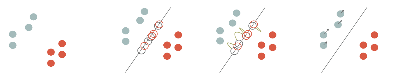
As mentioned above, the key tool will be Optimal Transport (OT for short) which can be sketched as follows: Given two probability (Radon) measures $\mu\in X$ and $\nu\in Y$, and a *cost function* $c(\cdot,\cdot): X\times Y \rightarrow \mathbb{R}^+$, an optimal transport plan $T: X\rightarrow Y$ minimizes
|
||
|
||
$${\displaystyle \inf \left\{\left.\int _{X}c(x,T(x))\,\mathrm {d} \mu (x)\;\right|\;T_{*}(\mu )=\nu \right\}.}$$
|
||
|
||
The cost of the optimal transport defines a metric between Radon measure. We can define the $p^{th}$ [Wasserstein metric](https://en.wikipedia.org/wiki/Wasserstein_metric), $\mathcal{W}_p(\mu,\nu)$ as
|
||
$$\displaystyle \mathcal{W}_{p}(\mu ,\nu ):={\left(\displaystyle \inf \left\{\left.\int _{X}c(x,T(x))^p\,\mathrm {d} \mu (x)\;\right|\;T_{*}(\mu )=\nu \right\}\right)^{1/p}}$$
|
||
|
||
An analogy with piles of sand is usually used to explain the definition: let us consider that $\mu$ is a pile of sand and $\nu$ a hole (with the same *volume* or *mass*), if we consider that the cost of moving an elementary volume of sand from on point to the other is proportional to the Euclidean distance ($l_2$ cost function), then the optimal transport plan gives you the most efficient way to move all the sand from $\mu$ to $\nu$. Again, the literature is huge and there are many alternative definitions, please refer to [Computational Optimal Transport](https://optimaltransport.github.io/book/) for a more complete introduction to the subject.
|
||
|
||
The link between OT and color transfer follows the observation that color histograms are discrete Radon measures. As we are looking for the *most efficient* transformation of the input image histogram to match with the target one, the color transfer problem can be reformulated as a discrete OT one [^b1][^b2][^b2b][^b3][^b4][^b5].
|
||
|
||
There are many numerical solutions to compute the OT (with continuous, discrete, semi-discrete measures, w/o regularization...). We focus here on the **sliced** formulation of the OT and associated 2-Wasserstein metric in dimension $d$:
|
||
|
||
$$ SW^2_2(\mu,\nu) := \int_{\mathbb{S}^d} \mathcal{W}_2^2( P_{\theta,\sharp}\mu,P_{\theta,\sharp}\nu) d\theta\,.$$
|
||
|
||
The sliced formulation consists in projecting the measures onto a 1D line ($P_{\theta,\sharp}: \mathbb{R}^d\rightarrow \mathbb{R}$), solving the 1D OT problem on the projections and average the results for all directions ($\mathbb{S}^d$ is the unit hypersphere in dimension $d$).
|
||
|
||
If the measures are discrete as the sums of Diracs centered at points $\{x_i\}$ and $\{y_i\}$ in $\mathbb{R}^d$ ($\mu := \frac{1}{n}\sum_{x_i} \delta_{x_i}$, $\nu := \frac{1}{n}\sum_{y_i} \delta_{y_i}$), then the 1D OT is obtained by sorting the projections and computing the difference between the first projected point of $\mu$ with the first projected point of $\nu$, the second with the second, etc...
|
||
|
||
$$ SW^2_2(\mu,\nu) = \int_{\mathbb{S}^d} \left(|\langle x_{\sigma_\theta(i)} - y_{\kappa_\theta(i)},\theta\rangle|^2 \right) d\theta\,,$$
|
||
($\sigma_\theta(i)$ a,d ${\kappa_\theta(i)}$ are permutations with increasing order).
|
||
|
||
Numerically, we sample the set of directions $\mathbb{S}^d$ and thus consider a finite number of *slices*.
|
||
|
||
# Sliced OT Color Transfer, the "TP"
|
||
|
||
Back to our histogram transfer problem, Diracs centers $\{x_i\}$ are points in RGB space (one Dirac per pixel of the input image), and $\{y_i\}$ are the colors of the target image. Matching the histogram can be seen a transportation of the point cloud $\mu$ to $\nu$ in $\mathbb{R^3}$ (the RGB color space).
|
||
|
||
The idea is to advect points of $\mu$ such that we minimize $SW(\mu,\nu)$. As described in the literature[^b1][^b2b][^b4], this amounts to project he points onto a random direction $\theta$, *align* the sorted projections and advect $\mu$ in the $\theta$ direction by $|\langle x_{\sigma_\theta(i)} - y_{\kappa_\theta(i)},\theta\rangle|$.
|
||
|
||
|
||
|
||
|
||
### The core
|
||
|
||
3. Get the `C++` / `python`. In Both cases, we provide elementary code to load/save RGB images. Please check how to access to RGB pixel values.
|
||
2. Create a function to draw a random direction
|
||
::: info
|
||
**Info**: to uniformly sample a direction in $\mathbb{R}^d$, a classical approach is to draw a $d$ dimensional random vector where each component follows a normal distribution (e.g. using C++ `std::normal_distribution`), with mean 0 and standard deviation equal to 1.0. Then normalize the vector and you have a uniform sampling of $\mathbb{S}^d$.
|
||
:::
|
||
3. From now on, the source (or target) image will be seen as a 3d point cloud in RGB space. Create a function to sort the projection of the samples of one image onto a random direction.
|
||
:::info
|
||
**Tip**: consider using a custom sort predicate in the C++ `std::sort` function.
|
||
:::
|
||
4. On this random direction $\theta$, sort both sample sets (source and target one) and advect the first sample, denoted $p_i$, of the source, along the $\theta$ direction, by an amount $d$ which correspond to the difference between projection of this first source sample, and the projection of the first target sample. In other words:
|
||
$$\vec{Op_i} = \vec{Op_i} + \langle x_{\sigma_\theta(0)} - y_{\kappa_\theta(0)},{\theta}\rangle ~{\theta}\,.$$
|
||
Do the same for the second ones, and the remaining samples.
|
||
|
||
:::info
|
||
**Tip**: Be careful when performing some computations on RGB `unsigned char` values. A good move would be to convert all data to `double` from the very beginning (and convert them back to `unsigned char` before exporting).
|
||
:::
|
||
|
||
5. Implement the main loop of the sliced approach: repeat the steps (draw a direction, sort the projections, compute the displacements, advect the source sample) until a maximum number of steps is reached.
|
||
6. To better set the maximum number of slices, output the sliced optimal transport energy with respect to the number of slices. You should also be able to *visualize* the convergence:
|
||
{%youtube FiVPXl3Io0w%}
|
||
|
||
### Advanced features
|
||
|
||
|
||
|
||
7. **Batches.** Instead of advecting $\mu$ for each $\theta$, we can accumulate advection vectors into a small batch and perform the transport step once the batch is full[^b4]. This corresponds to a stochastic gradient descent strategy in ML. Implement this "batch" approach. Compare this approach w.r.t to the legacy one (in terms of speed of convergence for instance).
|
||
8. **Regularization.** To obtain a smoother result or to be able to handle noise in the inputs, a classical approach consists in considering *regularized* optimal transport, or to regularize the optimal transport plan at the end of the computation. For color transfer, a simple way to mimic this approach consists in applying a non-linear smoothing filter to the transport plan[^b4]. A way to achieve this is to:
|
||
* once the sliced approach has converged, let's say we have a transformed source image $S^*$ of the image $S$ w.r.t. the target $T$;
|
||
* we express the transport plan as an *image* $(S^*-S)$;
|
||
* we can filter this image (using for instance a [bilateral filter](https://en.wikipedia.org/wiki/Bilateral_filter)) to obtain the final image : $\tilde{~S} = S + filter_\sigma(S^*-S)$.
|
||
|
||
:::info
|
||
**Tip**: In the `c++` project, we have included the [cimg](https://cimg.eu) header which contains an implementation of the bilateral filter. On `python`, the [OpenCV](https://opencv.org) package has been imported (which also contains an implementation of the bilateral filter).
|
||
:::
|
||
|
||
9. **Interpolation**: One can mimic the interpolation between two discrete measures in the sliced formulation by simply tweaking the advection step: instead of computing $\vec{Op_i} = \vec{Op_i} + \langle x_{\sigma_\theta(0)} - y_{\kappa_\theta(0)},{\theta}\rangle ~{\theta}$, just compute $\vec{Op_i} = \vec{Op_i} + \alpha\langle x_{\sigma_\theta(0)} - y_{\kappa_\theta(0)},{\theta}\rangle ~{\theta}$ for some $\alpha\in[0,1]$. You should be able to obtain something like that:
|
||
{%youtube Ti6kjJSdRnA%}
|
||
|
||
|
||
|
||
10. **Partial optimal transport**: as you may have noticed, the source and target images **must** have the same number of pixels. When the two discrete measures do not have the same number of Diracs, we are facing a *partial* optimal transport problem[^b6] (the overall all *sliced* approach remains the same, the 1D OT problem along the direcrtion is slightly more complicated). Without going to this *exact* partial solution, could you imagine and implement an approximate solution that *does the job* when the two images do not have the same size?
|
||
|
||
# References
|
||
|
||
[^b1]: Francois Pitié, Anil C. Kokaram, and Rozenn Dahyot. 2005. N-Dimensional Probablility Density Function Transfer and Its Application to Colour Transfer. In Proceedings of the Tenth IEEE International Conference on Computer Vision - Volume 2 (ICCV ’05). IEEE Computer Society, Washington, DC, USA, 1434–1439. https://doi.org/10.1109/ ICCV.2005.166
|
||
[^b2]: François Pitié, Anil C Kokaram, and Rozenn Dahyot. 2007. Automated colour grading using colour distribution transfer. Computer Vision and Image Understanding 107, 1-2 (2007), 123–137.
|
||
[^b2b]: Rabin Julien, Gabriel Peyré, Julie Delon, Bernot Marc, Wasserstein Barycenter and its Application to Texture Mixing. SSVM’11, 2011, Israel. pp.435-446. hal-00476064
|
||
[^b3]: Nicolas Bonneel, Julien Rabin, G. Peyré, and Hanspeter Pfister. 2015. Sliced and Radon Wasserstein Barycenters of Measures. J. of Mathematical Imaging and Vision 51, 1 (2015).
|
||
[^b4]: Julien Rabin, Julie Delon, and Yann Gousseau. 2010. Regularization of transportation maps for color and contrast transfer. In Image Processing (ICIP), 2010 17th IEEE International Conference on. IEEE, 1933–1936.
|
||
[^b5]: Nicolas Bonneel, Kalyan Sunkavalli, Sylvain Paris, and Hanspeter Pfister. 2013. Example- Based Video Color Grading. ACM Trans. Graph. (SIGGRAPH) 32, 4 (2013).
|
||
[^b6]: Nicolas Bonneel and David Coeurjolly. 2019. Sliced Partial Optimal Transport. ACM Trans. Graph. (SIGGRAPH) 38, 4 (2019).
|
||
|
||
|
||
|